Ships slow down for whales
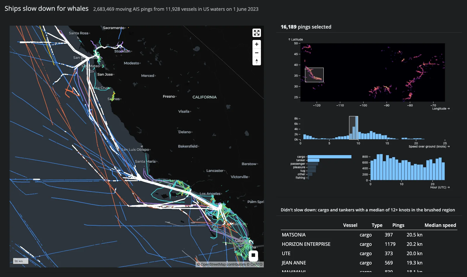
Every moving AIS ping from 11,928 vessels in US waters on a single day: 2,683,469 points in one lonboard ScatterplotLayer, crossfiltered by four Mosaic selections – a density map (region), a speed histogram, a vessel-type bar chart, and an hour-of-day histogram. Mosaic does the crossfiltering in DuckDB, so dragging a brush over millions of rows settles in about a second, and the selection flows back into Python, which highlights exactly those pings on the GPU map (an in-place layer swap; the 2.68M-point base layer is never re-sent).
The payoff is a real finding: brush the California coast, select cargo and tanker, and the speed histogram grows a spike just under 10 knots – the voluntary speed limit in the Santa Barbara Channel’s whale-protection zone. Brush the Gulf of Mexico instead and the spike is gone; the mode sits at about 12 knots, and the “Didn’t slow down” table names the vessels that kept up speed.
Run it
git clone --depth 1 https://github.com/posit-dev/py-shinywidgets
cd py-shinywidgets/website/gallery/showcases/whale-slowdown
uv run shiny run app.py
On first run the app downloads pings.parquet (~33 MB) from py-shinywidgets-data; prep_data.py rebuilds it from the raw NOAA CSV. There is no Shinylive link: DuckDB and a 33 MB download don’t belong in a browser tab.
Source: app.py
Try this
- Find the spike. Drag a box around California on the density map (top right). Click cargo in the vessel-type bars, then shift-click tanker. The speed histogram grows a spike just under 10 kn, and the map flies to your brush.
- Brush the spike. Brush roughly 8.5-10 kn on the speed histogram. White pings trace the Santa Barbara Channel and the San Francisco approach lanes: the ships that slowed down, and exactly where.
- Compare the Gulf. Click outside the box to clear it, then draw a new box over the Gulf of Mexico. The spike is gone – the hump is at about 12 kn, and the table names the fast cargo ships and tankers in that region.
Gestures: drag to brush, drag inside a box to move it, click outside a box to clear it, shift-click the type bars to select several.
Techniques demonstrated
- Mosaic params as a reactive input. The widget’s
paramstrait carries all four selections; a 300 ms debounce collapses a drag, andw.data("pings", filter_by=[...])asks Mosaic for the selected rows as a DuckDB relation – the caption, the map highlight, and the slowpoke table all read the same debounced selection. - In-place highlight on a huge layer. The selection becomes a second
ScatterplotLayerswapped intomap.widget.layers(sampled to 300k points when the selection is larger): 300k rows cross the wire in ~0.4 s while the 2.68M-point base layer stays put. - Brush-to-fly-to. When the region brush settles, its lon/lat bounds become a
map.widget.fly_to(...); clearing the brush flies back to the full US view.
Verification
Driven end-to-end with Playwright on the hosted parquet: a California brush selecting cargo+tanker puts the speed mode in the 9.5-10 kn bin (8,940 pings) and a Gulf brush puts it at 12 kn, matching the independently computed DuckDB counts (2,683,469 pings from 11,928 vessels). First paint is ~5.5 s with 43 MB over the websocket; a rapid 30-step brush settles within 1 s. See img/hero.webp, captured mid-story: California cargo and tankers brushed, spike visible just under 10 kn.